使用 Informer 进行多元概率时间序列预测

介绍

几个月前，我们介绍了 Time Series Transformer，它是 Vanilla Transformer (Vaswani et al., 2017) 应用于预测的模型，并展示了单变量概率预测任务的示例（即单独预测每个时间序列的 1-d 分布）。在这篇文章中，我们介绍了 Informer 模型 (Zhou, Haoyi, et al., 2021)，AAAI21最佳论文，现在在🤗 Transformers 中 可用。我们将展示如何使用 Informer 模型进行 多元 概率时间序列预测任务，即预测未来时间序列目标值的 向量 的分布。请注意，这也适用于原始时间序列 Transformer 模型。

多元概率时间序列预测

就概率预测的建模方面而言，当处理多元时间序列时，Transformer/Informer 不需要进行任何更改。在单变量和多变量设置中，模型将接收一系列向量，因此唯一的更改在于最终输出或模型输出。

对高维数据的完整联合条件分布进行建模可能会使得计算变得非常昂贵，因此会采用某些分布的近似方法，最简单的是将数据建模为来自相同族的独立分布，或者是对完整协方差的某些低秩近似等。在这里，我们将只使用独立（或对角线）模型输出，这些模型输出受到我们已实现的分布族支持。

Informer – 原理

基于原始 Transformer（Vaswani et al., 2017），Informer 采用了两个主要改进。为了理解这些改进，让我们回顾一下原始 Transformer 的缺点：

1. 规范自注意力机制的二次计算： 原始 Transformer 的计算复杂度为 \(O(T^2 D)\) ，其中 \(T\) 是时间序列长度，\(D\) 是隐藏状态的维度。对于长序列时间序列预测（也称为 LSTF 问题 ），可能非常耗费计算资源。为了解决这个问题，Informer 采用了一种新的自注意力机制，称为 稀疏概率 自注意力机制，其时间和空间复杂度为 \(O(T \log T)\)。
2. 堆叠层时的内存瓶颈：当堆叠 \(N\) 个编码器/解码器层时，原始 Transformer 的内存使用量为 \(O(N T^2)\)，这限制了模型对长序列的容量。Informer 使用了一种称为 蒸馏 操作的方法，将层之间的输入大小缩小到其一半切片。通过这样做，它将整个内存使用量减少到 \(O(N\cdot T \log T)\)。

正如您所看到的，Informer 模型的原理类似于 Longformer（Beltagy et el., 2020），Sparse Transformer（Child et al., 2019）和其他 NLP 论文，当输入序列很长时用于减少自注意力机制的二次复杂度。现在，让我们深入了解 稀疏概率 自注意力机制 和 蒸馏 操作，并提供代码示例。

稀疏概率自注意力机制（ProbSparse attention）

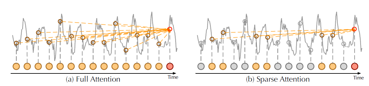
稀疏概率的主要思想是规范的自注意力分数形成长尾分布，其中“激活” query 位于“头部”分数，“沉默” query 位于“尾部”区域的分数。通过“激活” query，我们的意思是 query \(q_i\) 这样点积 \(\langle q_i,k_i \rangle\) 有助于主要的注意力，而“沉默” query 形成一个点积，产生 琐碎的 注意力。这里，\(q_i\) 和 \(k_i\) 分别是 \(Q\) 和 \(K\) 注意力矩阵中的第 \(i\) 行。

在 Autoformer (Wu, Haixu, et al., 2021)中，原始自注意力机制 vs 稀疏概率自注意力机制

基于“激活”和“沉默” query 的想法，稀疏概率自注意力机制选择“激活” query ，并创建一个简化的 query 矩阵 \(Q_{reduced}\) 用于计算 \ 中的注意力权重(O(T \log T)\)。让我们通过代码示例更详细地了解这一点。

回忆一下典型的自注意力公式：

$$
\textrm{Attention}(Q, K, V) = \textrm{softmax}(\frac{QK^T}{\sqrt{d_k}} )V
$$

其中 \(Q\in \mathbb{R}^{L_Q \times d}\)、\(K\in \mathbb{R}^{L_K \times d}\) 和 \(V\in \mathbb{R}^{L_V \times d}\)。请注意，在实践中，query 和 key 的输入长度在自注意力计算中通常是等效的，即 \(L_Q = LK = T\) 其中 \(T\) 是时间序列长度。因此，\(QK^T\) 乘法需要 \(O(T^2 \cdot d)\) 计算复杂度。在稀疏概率自注意力机制中，我们的目标是创建一个新的 \(Q{reduce}\) 矩阵并定义：

$$
\textrm{ProbSparseAttention}(Q, K, V) = \textrm{softmax}(\frac{Q_{reduce}K^T}{\sqrt{d_k}} )V
$$

其中 \(Q_{reduce}\) 矩阵仅选择 Top \(u\) 个“激活” query 。这里，\(u = c \cdot \log L_Q\) 和 \(c\) 调用了稀疏概率自注意力机制的 采样因子 超参数。由于 \(Q_{reduce}\) 仅选择 Top \(u\) query，其大小为 \(c\cdot \log LQ \times d\)，因此乘法 \(Q {reduce}K^T\) 只需要 \(O(L_K \log L_Q) = O(T \log T)\)。

这很好！但是我们如何选择 \(u\) 个“激活” query 来创建 \(Q_{reduce}\)？让我们定义 Query 稀疏度测量(Query Sparsity Measurement)。

Query 稀疏度测量(Query Sparsity Measurement)

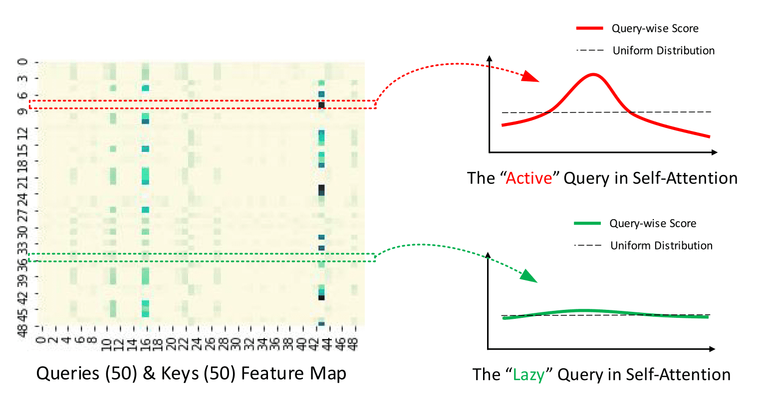
Query 稀疏度测量 \(M(q_i, K)\) 用于在 \(Q\) 中选择 \(u\) “激活” query \(qi\) 以创建 \ （Q{reduce}\）。从理论上讲，占主导地位的 \(\langle q_i,k_i \rangle\) 对鼓励“激活” \(q_i\) 的概率分布远离均匀分布，如下图所示。因此，实际 query 分布与均匀分布之间的 KL 散度 用于定义稀疏度度量。

从官方仓库 给出的稀疏概率自注意力机制描述

实际中，测量被定义为：

$$
M(q_i, K) = \max_j \frac{q_ik_j^T}{\sqrt{d}}-\frac{1}{Lk} \sum{j=1}^{L_k}\frac{q_ik_j^T}{\sqrt{d}}
$$

这里要理解的重要一点是当 \(M(q_i, K)\) 较大时，Query \(qi\) 应该在 \(Q{reduce}\) 中，反之亦然。

但是我们如何计算非二次时间的项 \(q_ik_j^T\) 呢？回想一下，大多数点积 \(\langle q_i,k_i \rangle\) 都会产生正常的注意力（即长尾分布属性），所以从 \(K\) 中随机抽取一个键子集就足够了，这在代码中称为 K_sample。

现在，我们来看一看 probsparse_attention 的代码：

from torch import nn
import math

def probsparse_attention(query_states, key_states, value_states, sampling_factor=5):
    """
    Compute the probsparse self-attention.
    Input shape: Batch x Time x Channel

    Note the additional `sampling_factor` input.
    """
    # get input sizes with logs
    L_K = key_states.size(1)
    L_Q = query_states.size(1)
    log_L_K = np.ceil(np.log1p(L_K)).astype("int").item()
    log_L_Q = np.ceil(np.log1p(L_Q)).astype("int").item()

    # calculate a subset of samples to slice from K and create Q_K_sample
    U_part = min(sampling_factor * L_Q * log_L_K, L_K)

    # create Q_K_sample (the q_i * k_j^T term in the sparsity measurement)
    index_sample = torch.randint(0, L_K, (U_part,))
    K_sample = key_states[:, index_sample, :]
    Q_K_sample = torch.bmm(query_states, K_sample.transpose(1, 2))

    # calculate the query sparsity measurement with Q_K_sample
    M = Q_K_sample.max(dim=-1)[0] - torch.div(Q_K_sample.sum(dim=-1), L_K)

    # calculate u to find the Top-u queries under the sparsity measurement
    u = min(sampling_factor * log_L_Q, L_Q)
    M_top = M.topk(u, sorted=False)[1]

    # calculate Q_reduce as query_states[:, M_top]
    dim_for_slice = torch.arange(query_states.size(0)).unsqueeze(-1)
    Q_reduce = query_states[dim_for_slice, M_top]  # size: c*log_L_Q x channel

    # and now, same as the canonical
    d_k = query_states.size(-1)
    attn_scores = torch.bmm(Q_reduce, key_states.transpose(-2, -1))  # Q_reduce x K^T
    attn_scores = attn_scores / math.sqrt(d_k)
    attn_probs = nn.functional.softmax(attn_scores, dim=-1)
    attn_output = torch.bmm(attn_probs, value_states)

    return attn_output, attn_scores

我们做到了！请注意，这只是 probsparse_attention 的部分实现，完整的实现可以在 🤗 Transformers 中找到。

蒸馏(distilling)

由于概率稀疏自注意力机制，编码器的特征图有一些可以去除的冗余。所以，
蒸馏操作用于将编码器层之间的输入大小减少到它的半片，从而在理论上消除了这种冗余。实际上，Informer 的“蒸馏”操作只是在每个编码器层之间添加一维卷积层和最大池化。设 \(X_n\) 为第 \(n\) 编码层的输出，则蒸馏操作定义为：

$$
X_{n+1} = \textrm{MaxPool} ( \textrm{ELU}(\textrm{Conv1d}(X_n))
$$

让我们看一下代码：

from torch import nn

# ConvLayer is a class with forward pass applying ELU and MaxPool1d
def informer_encoder_forward(x_input, num_encoder_layers=3, distil=True):
    # Initialize the convolution layers
    if distil:
        conv_layers = nn.ModuleList([ConvLayer() for _ in range(num_encoder_layers - 1)])
        conv_layers.append(None)
    else:
        conv_layers = [None] * num_encoder_layers

    # Apply conv_layer between each encoder_layer
    for encoder_layer, conv_layer in zip(encoder_layers, conv_layers):
        output = encoder_layer(x_input)
        if conv_layer is not None:
            output = conv_layer(loutput)

    return output

通过将每层的输入减少两个，我们得到的内存使用量为 \(O(N\cdot T \log T)\) 而不是 \(O(N\cdot T^2)\) 其中\(N\) 是编码器/解码器层数。这就是我们想要的！

Informer 模型在 🤗 Transformers 库中 现已可用，简称为 InformerModel。在下面的部分中，我们将展示如何在自定义多元时间序列数据集上训练此模型。

设置环境

首先，让我们安装必要的库：🤗 Transformers、🤗 Datasets、🤗 Evaluate、🤗 Accelerate 和 GluonTS。

正如我们将展示的那样，GluonTS 将用于转换数据以创建特征以及创建适当的训练、验证和测试批次。

!pip install -q git+https://github.com/huggingface/transformers.git datasets evaluate accelerate gluonts ujson

加载数据集

在这篇博文中，我们将使用 Hugging Face Hub 上提供的 traffic_hourly 数据集。该数据集包含 Lai 等人使用的旧金山交通数据集。 (2017)。它包含 862 个小时的时间序列，显示 2015 年至 2016 年旧金山湾区高速公路 \([0, 1]\) 范围内的道路占用率。

此数据集是 Monash Time Series Forecasting 仓库的一部分，该仓库是来自多个领域的时间序列数据集的集合。它可以被视为时间序列预测的 GLUE 基准。

from datasets import load_dataset

dataset = load_dataset("monash_tsf", "traffic_hourly")

可以看到，数据集包含 3 个切片：训练集，验证集，测试集。

dataset

>>> DatasetDict({
        train: Dataset({
            features: ['start', 'target', 'feat_static_cat', 'feat_dynamic_real', 'item_id'],
            num_rows: 862
        })
        test: Dataset({
            features: ['start', 'target', 'feat_static_cat', 'feat_dynamic_real', 'item_id'],
            num_rows: 862
        })
        validation: Dataset({
            features: ['start', 'target', 'feat_static_cat', 'feat_dynamic_real', 'item_id'],
            num_rows: 862
        })
    })

每个示例都包含一些键，其中 start和 target 是最重要的键。让我们看一下数据集中的第一个时间序列：

train_example = dataset["train"][0]
train_example.keys()

>>> dict_keys(['start', 'target', 'feat_static_cat', 'feat_dynamic_real', 'item_id'])

start 仅指示时间序列的开始（作为日期时间），而 ta​​rget 包含时间序列的实际值。

start 将有助于将时间相关的特征添加到时间序列值中，作为模型的额外输入（例如“一年中的月份”）。因为我们知道数据的频率是每小时，所以我们知道例如第二个值的时间戳为2015-01-01 01:00:01、2015-01-01 02:00:01 等等。

print(train_example["start"])
print(len(train_example["target"]))

>>> 2015-01-01 00:00:01
    17448

验证集包含与训练集相同的数据，只是 prediction_length 的时间更长。这使我们能够根据真实情况验证模型的预测。

与验证集相比，测试集也是一个 prediction_length 长数据（或者与用于在多个滚动窗口上进行测试的训练集相比，prediction_length 长数据的若干倍）。

validation_example = dataset["validation"][0]
validation_example.keys()

>>> dict_keys(['start', 'target', 'feat_static_cat', 'feat_dynamic_real', 'item_id'])

初始值与相应的训练示例完全相同。但是，与训练示例相比，此示例具有 prediction_length=48（48 小时或 2 天）附加值。让我们验证一下。

freq = "1H"
prediction_length = 48

assert len(train_example["target"]) + prediction_length == len(
    dataset["validation"][0]["target"]
)

让我们可视化看一下：

import matplotlib.pyplot as plt

num_of_samples = 150

figure, axes = plt.subplots()
axes.plot(train_example["target"][-num_of_samples:], color="blue")
axes.plot(
    validation_example["target"][-num_of_samples - prediction_length :],
    color="red",
    alpha=0.5,
)

plt.show()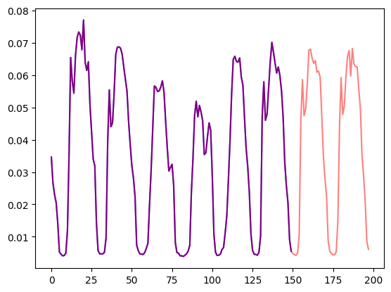

让我们划分一下数据：

train_dataset = dataset["train"]
test_dataset = dataset["test"]

更新 start 到 pd.Period

我们要做的第一件事是使用数据的 freq 将每个时间序列的 start 特征转换为 pandas Period 索引：

from functools import lru_cache

import pandas as pd
import numpy as np

@lru_cache(10_000)
def convert_to_pandas_period(date, freq):
    return pd.Period(date, freq)

def transform_start_field(batch, freq):
    batch["start"] = [convert_to_pandas_period(date, freq) for date in batch["start"]]
    return batch

我们现在使用 datasets‘ set_transform 功能来即时执行此操作到位：

from functools import partial

train_dataset.set_transform(partial(transform_start_field, freq=freq))
test_dataset.set_transform(partial(transform_start_field, freq=freq))

现在，让我们使用 GluonTS 中的 MultivariateGrouper 将数据集转换为多元时间序列。该 grouper 会将单个一维时间序列转换为单个二维矩阵。

from gluonts.dataset.multivariate_grouper import MultivariateGrouper

num_of_variates = len(train_dataset)

train_grouper = MultivariateGrouper(max_target_dim=num_of_variates)
test_grouper = MultivariateGrouper(
    max_target_dim=num_of_variates,
    num_test_dates=len(test_dataset) // num_of_variates, # number of rolling test windows
)

multi_variate_train_dataset = train_grouper(train_dataset)
multi_variate_test_dataset = test_grouper(test_dataset)

请注意，目标现在是二维的，其中第一个维度是变量的数量（时间序列的数量），第二个是时间序列值（时间维度）：

multi_variate_train_example = multi_variate_train_dataset[0]
print("multi_variate_train_example["target"].shape =", multi_variate_train_example["target"].shape)

>>> multi_variate_train_example["target"].shape = (862, 17448)

定义模型

接下来，让我们实例化一个模型。该模型将从头开始训练，因此我们不会在这里使用 from_pretrained 方法，而是从 config 随机初始化模型。

我们为模型指定了几个附加参数：

• prediction_length (在我们的例子中, 48 小时): 这是 Informer 的解码器将学习预测的范围；
• context_length: 如果未指定 context_length ，模型会将 context_length （编码器的输入）设置为等于 prediction_length；
• 给定频率的 lags : 这些指定了一种有效的“回顾”机制，我们将过去的值连接到当前值作为附加功能，例如对于每日频率，我们可能会考虑回顾[1, 7, 30, ...]，或者对于分钟数据，我们可能会考虑[1, 30, 60, 60*24, ... ] 等；
• 时间特征的数量: 在我们的例子中，这将是 5，因为我们将添加 HourOfDay、DayOfWeek …… 和 Age 特征（见下文）。

让我们检查 GluonTS 为给定频率（“每小时”）提供的默认 lags：

from gluonts.time_feature import get_lags_for_frequency

lags_sequence = get_lags_for_frequency(freq)
print(lags_sequence)

>>> [1, 2, 3, 4, 5, 6, 7, 23, 24, 25, 47, 48, 49, 71, 72, 73, 95, 96, 97, 119, 120, 
     121, 143, 144, 145, 167, 168, 169, 335, 336, 337, 503, 504, 505, 671, 672, 673, 719, 720, 721]

这意味着每个时间步长最多可回顾 721 小时（约 30 天），作为附加功能。但是，生成的特征向量最终的大小为 len(lags_sequence)*num_of_variates，对于我们的例子来说是 34480！这是行不通的，所以我们将使用我们自己的合理滞后。

我们还检查 GluonTS 为我们提供的默认时间功能：

from gluonts.time_feature import time_features_from_frequency_str

time_features = time_features_from_frequency_str(freq)
print(time_features)

>>> [<function hour_of_day at 0x7f3809539240>, <function day_of_week at 0x7f3809539360>, <function day_of_month at 0x7f3809539480>, <function day_of_year at 0x7f38095395a0>]

在这种情况下，有四个附加特征，即“一天中的小时”、“星期几”、“月中的天”和“年中的天”。这意味着对于每个时间步，我们将这些特征添加为标量值。例如，考虑时间戳 2015-01-01 01:00:01。四个附加函数是：

from pandas.core.arrays.period import period_array

timestamp = pd.Period("2015-01-01 01:00:01", freq=freq)
timestamp_as_index = pd.PeriodIndex(data=period_array([timestamp]))
additional_features = [
    (time_feature.__name__, time_feature(timestamp_as_index))
    for time_feature in time_features
]
print(dict(additional_features))

>>> {'hour_of_day': array([-0.45652174]), 'day_of_week': array([0.]), 'day_of_month': array([-0.5]), 'day_of_year': array([-0.5])}

请注意，小时和天被编码为来自 GluonTS 的[-0.5, 0.5]之间的值。有关 time_features 的更多信息，请参阅这里。除了这 4 个特征之外，我们还将添加一个“年龄”特征，我们将在稍后的数据 transformations 中看到这一点。

我们现在拥有了定义模型的一切：

from transformers import InformerConfig, InformerForPrediction

config = InformerConfig(
    # in the multivariate setting, input_size is the number of variates in the time series per time step
    input_size=num_of_variates,
    # prediction length:
    prediction_length=prediction_length,
    # context length:
    context_length=prediction_length * 2,
    # lags value copied from 1 week before:
    lags_sequence=[1, 24 * 7],
    # we'll add 5 time features ("hour_of_day", ..., and "age"):
    num_time_features=len(time_features) + 1,

    # informer params:
    dropout=0.1,
    encoder_layers=6,
    decoder_layers=4,
    # project input from num_of_variates*len(lags_sequence)+num_time_features to:
    d_model=64,
)

model = InformerForPrediction(config)

默认情况下，该模型使用对角 Student-t 分布（但这是 可配置的）：

model.config.distribution_output

>>> 'student_t'

定义 Transformations

接下来，我们定义数据的 transformations，特别是时间特征的创建（基于数据集或通用数据集）。

同样，我们将为此使用 GluonTS 库。我们定义了一个 transformations 链（有点类似于图像的 torchvision.transforms.Compose）。它允许我们将多个 transformations 组合到一个 pipeline 中。

from gluonts.time_feature import TimeFeature
from gluonts.dataset.field_names import FieldName
from gluonts.transform import (
    AddAgeFeature,
    AddObservedValuesIndicator,
    AddTimeFeatures,
    AsNumpyArray,
    Chain,
    ExpectedNumInstanceSampler,
    InstanceSplitter,
    RemoveFields,
    SelectFields,
    SetField,
    TestSplitSampler,
    Transformation,
    ValidationSplitSampler,
    VstackFeatures,
    RenameFields,
)

下面的 transformations 带有注释，以解释它们的作用。在高层次上，我们将迭代数据集的各个时间序列并添加/删除字段或特征：

from transformers import PretrainedConfig

def create_transformation(freq: str, config: PretrainedConfig) -> Transformation:
    # create list of fields to remove later
    remove_field_names = []
    if config.num_static_real_features == 0:
        remove_field_names.append(FieldName.FEAT_STATIC_REAL)
    if config.num_dynamic_real_features == 0:
        remove_field_names.append(FieldName.FEAT_DYNAMIC_REAL)
    if config.num_static_categorical_features == 0:
        remove_field_names.append(FieldName.FEAT_STATIC_CAT)

    return Chain(
        # step 1: remove static/dynamic fields if not specified
        [RemoveFields(field_names=remove_field_names)]
        # step 2: convert the data to NumPy (potentially not needed)
        + (
            [
                AsNumpyArray(
                    field=FieldName.FEAT_STATIC_CAT,
                    expected_ndim=1,
                    dtype=int,
                )
            ]
            if config.num_static_categorical_features > 0
            else []
        )
        + (
            [
                AsNumpyArray(
                    field=FieldName.FEAT_STATIC_REAL,
                    expected_ndim=1,
                )
            ]
            if config.num_static_real_features > 0
            else []
        )
        + [
            AsNumpyArray(
                field=FieldName.TARGET,
                # we expect an extra dim for the multivariate case:
                expected_ndim=1 if config.input_size == 1 else 2,
            ),
            # step 3: handle the NaN's by filling in the target with zero
            # and return the mask (which is in the observed values)
            # true for observed values, false for nan's
            # the decoder uses this mask (no loss is incurred for unobserved values)
            # see loss_weights inside the xxxForPrediction model
            AddObservedValuesIndicator(
                target_field=FieldName.TARGET,
                output_field=FieldName.OBSERVED_VALUES,
            ),
            # step 4: add temporal features based on freq of the dataset
            # these serve as positional encodings
            AddTimeFeatures(
                start_field=FieldName.START,
                target_field=FieldName.TARGET,
                output_field=FieldName.FEAT_TIME,
                time_features=time_features_from_frequency_str(freq),
                pred_length=config.prediction_length,
            ),
            # step 5: add another temporal feature (just a single number)
            # tells the model where in the life the value of the time series is
            # sort of running counter
            AddAgeFeature(
                target_field=FieldName.TARGET,
                output_field=FieldName.FEAT_AGE,
                pred_length=config.prediction_length,
                log_scale=True,
            ),
            # step 6: vertically stack all the temporal features into the key FEAT_TIME
            VstackFeatures(
                output_field=FieldName.FEAT_TIME,
                input_fields=[FieldName.FEAT_TIME, FieldName.FEAT_AGE]
                + (
                    [FieldName.FEAT_DYNAMIC_REAL]
                    if config.num_dynamic_real_features > 0
                    else []
                ),
            ),
            # step 7: rename to match HuggingFace names
            RenameFields(
                mapping={
                    FieldName.FEAT_STATIC_CAT: "static_categorical_features",
                    FieldName.FEAT_STATIC_REAL: "static_real_features",
                    FieldName.FEAT_TIME: "time_features",
                    FieldName.TARGET: "values",
                    FieldName.OBSERVED_VALUES: "observed_mask",
                }
            ),
        ]
    )

定义 InstanceSplitter

为了训练/验证/测试，我们接下来创建一个 InstanceSplitter，用于从数据集中对窗口进行采样（因为，请记住，由于时间和内存限制，我们无法将整个历史值传递给模型）。

实例拆分器从数据中随机采样大小为 context_length 和后续大小为prediction_length 的窗口，并将 past_ 或 future_键附加到各个窗口的任何时间键。这确保了 values 将被拆分为 past_values 和后续的 future_values 键，它们将分别用作编码器和解码器的输入。 time_series_fields 参数中的任何键都会发生同样的情况：

from gluonts.transform.sampler import InstanceSampler
from typing import Optional

def create_instance_splitter(
    config: PretrainedConfig,
    mode: str,
    train_sampler: Optional[InstanceSampler] = None,
    validation_sampler: Optional[InstanceSampler] = None,
) -> Transformation:
    assert mode in ["train", "validation", "test"]

    instance_sampler = {
        "train": train_sampler
        or ExpectedNumInstanceSampler(
            num_instances=1.0, min_future=config.prediction_length
        ),
        "validation": validation_sampler
        or ValidationSplitSampler(min_future=config.prediction_length),
        "test": TestSplitSampler(),
    }[mode]

    return InstanceSplitter(
        target_field="values",
        is_pad_field=FieldName.IS_PAD,
        start_field=FieldName.START,
        forecast_start_field=FieldName.FORECAST_START,
        instance_sampler=instance_sampler,
        past_length=config.context_length + max(config.lags_sequence),
        future_length=config.prediction_length,
        time_series_fields=["time_features", "observed_mask"],
    )

创建 PyTorch DataLoaders

下面是时候创建 PyTorch DataLoaders 了,这将允许我们这允许我们拥有成批的（输入、输出）对——或者换句话说（past_values、future_values）。

from typing import Iterable

import torch
from gluonts.itertools import Cached, Cyclic
from gluonts.dataset.loader import as_stacked_batches

def create_train_dataloader(
    config: PretrainedConfig,
    freq,
    data,
    batch_size: int,
    num_batches_per_epoch: int,
    shuffle_buffer_length: Optional[int] = None,
    cache_data: bool = True,
    **kwargs,
) -> Iterable:
    PREDICTION_INPUT_NAMES = [
        "past_time_features",
        "past_values",
        "past_observed_mask",
        "future_time_features",
    ]
    if config.num_static_categorical_features > 0:
        PREDICTION_INPUT_NAMES.append("static_categorical_features")

    if config.num_static_real_features > 0:
        PREDICTION_INPUT_NAMES.append("static_real_features")

    TRAINING_INPUT_NAMES = PREDICTION_INPUT_NAMES + [
        "future_values",
        "future_observed_mask",
    ]

    transformation = create_transformation(freq, config)
    transformed_data = transformation.apply(data, is_train=True)
    if cache_data:
        transformed_data = Cached(transformed_data)

    # we initialize a Training instance
    instance_splitter = create_instance_splitter(config, "train")

    # the instance splitter will sample a window of
    # context length + lags + prediction length (from all the possible transformed time series, 1 in our case)
    # randomly from within the target time series and return an iterator.
    stream = Cyclic(transformed_data).stream()
    training_instances = instance_splitter.apply(
        stream, is_train=True
    )

    return as_stacked_batches(
        training_instances,
        batch_size=batch_size,
        shuffle_buffer_length=shuffle_buffer_length,
        field_names=TRAINING_INPUT_NAMES,
        output_type=torch.tensor,
        num_batches_per_epoch=num_batches_per_epoch,
    )

def create_test_dataloader(
    config: PretrainedConfig,
    freq,
    data,
    batch_size: int,
    **kwargs,
):
    PREDICTION_INPUT_NAMES = [
        "past_time_features",
        "past_values",
        "past_observed_mask",
        "future_time_features",
    ]
    if config.num_static_categorical_features > 0:
        PREDICTION_INPUT_NAMES.append("static_categorical_features")

    if config.num_static_real_features > 0:
        PREDICTION_INPUT_NAMES.append("static_real_features")

    transformation = create_transformation(freq, config)
    transformed_data = transformation.apply(data, is_train=False)

    # we create a Test Instance splitter which will sample the very last
    # context window seen during training only for the encoder.
    instance_sampler = create_instance_splitter(config, "test")

    # we apply the transformations in test mode
    testing_instances = instance_sampler.apply(transformed_data, is_train=False)

    return as_stacked_batches(
        testing_instances,
        batch_size=batch_size,
        output_type=torch.tensor,
        field_names=PREDICTION_INPUT_NAMES,
    )

train_dataloader = create_train_dataloader(
    config=config,
    freq=freq,
    data=multi_variate_train_dataset,
    batch_size=256,
    num_batches_per_epoch=100,
    num_workers=2,
)

test_dataloader = create_test_dataloader(
    config=config,
    freq=freq,
    data=multi_variate_test_dataset,
    batch_size=32,
)

让我们查看一下第一批次：

batch = next(iter(train_dataloader))
for k, v in batch.items():
    print(k, v.shape, v.type())

>>> past_time_features torch.Size([256, 264, 5]) torch.FloatTensor
    past_values torch.Size([256, 264, 862]) torch.FloatTensor
    past_observed_mask torch.Size([256, 264, 862]) torch.FloatTensor
    future_time_features torch.Size([256, 48, 5]) torch.FloatTensor
    future_values torch.Size([256, 48, 862]) torch.FloatTensor
    future_observed_mask torch.Size([256, 48, 862]) torch.FloatTensor

可以看出，我们没有将 input_ids 和 attention_mask 提供给编码器（NLP 模型就是这种情况），而是将 past_values 以及 past_observed_mask、past_time_features 和 static_real_features 提供给编码器.

解码器输入包括 future_values、future_observed_mask 和 future_time_features。 future_values 可以等同于 NLP 中的 decoder_input_ids 。

我们参考了文档 以获得对它们中每一个的详细解释。

前向传递

让我们对刚刚创建的批次执行一次前向传递：

# perform forward pass
outputs = model(
    past_values=batch["past_values"],
    past_time_features=batch["past_time_features"],
    past_observed_mask=batch["past_observed_mask"],
    static_categorical_features=batch["static_categorical_features"]
    if config.num_static_categorical_features > 0
    else None,
    static_real_features=batch["static_real_features"]
    if config.num_static_real_features > 0
    else None,
    future_values=batch["future_values"],
    future_time_features=batch["future_time_features"],
    future_observed_mask=batch["future_observed_mask"],
    output_hidden_states=True,
)

print("Loss:", outputs.loss.item())

>>> Loss: -1071.5718994140625

请注意，该模型正在返回损失。这是可能的，因为解码器会自动将 future_values 向右移动一个位置以获得标签。这将允许计算预测值和标签之间的损失。损失是预测分布相对于真实值的负对数似然，并且趋于负无穷大。

另外请注意，解码器使用因果掩码来遮盖未来，因为它需要预测的值在 future_values 张量中。

训练模型

是时候训练模型了！我们将会使用标准的 PyTorch training loop。

我们将在这里使用 🤗 Accelerate 库，它会自动将模型、优化器和数据加载器放置在适当的设备上。

from accelerate import Accelerator
from torch.optim import AdamW

epochs = 25
loss_history = []

accelerator = Accelerator()
device = accelerator.device

model.to(device)
optimizer = AdamW(model.parameters(), lr=6e-4, betas=(0.9, 0.95), weight_decay=1e-1)

model, optimizer, train_dataloader = accelerator.prepare(
    model,
    optimizer,
    train_dataloader,
)

model.train()
for epoch in range(epochs):
    for idx, batch in enumerate(train_dataloader):
        optimizer.zero_grad()
        outputs = model(
            static_categorical_features=batch["static_categorical_features"].to(device)
            if config.num_static_categorical_features > 0
            else None,
            static_real_features=batch["static_real_features"].to(device)
            if config.num_static_real_features > 0
            else None,
            past_time_features=batch["past_time_features"].to(device),
            past_values=batch["past_values"].to(device),
            future_time_features=batch["future_time_features"].to(device),
            future_values=batch["future_values"].to(device),
            past_observed_mask=batch["past_observed_mask"].to(device),
            future_observed_mask=batch["future_observed_mask"].to(device),
        )
        loss = outputs.loss

        # Backpropagation
        accelerator.backward(loss)
        optimizer.step()

        loss_history.append(loss.item())
        if idx % 100 == 0:
            print(loss.item())

>>> -1081.978515625
    ...
    -2877.723876953125

# view training
loss_history = np.array(loss_history).reshape(-1)
x = range(loss_history.shape[0])
plt.figure(figsize=(10, 5))
plt.plot(x, loss_history, label="train")
plt.title("Loss", fontsize=15)
plt.legend(loc="upper right")
plt.xlabel("iteration")
plt.ylabel("nll")
plt.show()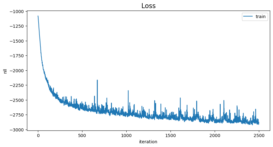

推理

在推理时，建议使用 generate() 方法进行自回归生成，类似于 NLP 模型。

预测涉及从测试实例采样器获取数据，该采样器将从数据集中每个时间序列的最后一个 context_length 大小的值窗口中采样，并将其传递给模型。请注意，我们将提前已知的 future_time_features 传递给解码器。

该模型将从预测分布中自回归采样一定数量的值，并将它们传回解码器以返回预测输出：

model.eval()

forecasts_ = []

for batch in test_dataloader:
    outputs = model.generate(
        static_categorical_features=batch["static_categorical_features"].to(device)
        if config.num_static_categorical_features > 0
        else None,
        static_real_features=batch["static_real_features"].to(device)
        if config.num_static_real_features > 0
        else None,
        past_time_features=batch["past_time_features"].to(device),
        past_values=batch["past_values"].to(device),
        future_time_features=batch["future_time_features"].to(device),
        past_observed_mask=batch["past_observed_mask"].to(device),
    )
    forecasts_.append(outputs.sequences.cpu().numpy())

该模型输出形状的张量（batch_size、number of samples、prediction length、input_size）。

在这种情况下，对于 862 时间序列中的每个时间序列，我们在接下来的 48 小时内获得 100 个可能值（对于大小为 1 的批处理中的每个示例，因为我们只有一个多元时间序列）：

forecasts_[0].shape

>>> (1, 100, 48, 862)

我们将垂直堆叠它们，以获得测试数据集中所有时间序列的预测（以防万一测试集中有更多时间序列）：

forecasts = np.vstack(forecasts_)
print(forecasts.shape)

>>> (1, 100, 48, 862)

我们可以根据测试集中存在的样本值，根据真实情况评估生成的预测。为此，我们将使用 🤗 Evaluate 库，其中包括 MASE 和 sMAPE 指标。

我们计算数据集中每个时间序列变量的两个指标：

from evaluate import load
from gluonts.time_feature import get_seasonality

mase_metric = load("evaluate-metric/mase")
smape_metric = load("evaluate-metric/smape")

forecast_median = np.median(forecasts, 1).squeeze(0).T

mase_metrics = []
smape_metrics = []

for item_id, ts in enumerate(test_dataset):
    training_data = ts["target"][:-prediction_length]
    ground_truth = ts["target"][-prediction_length:]
    mase = mase_metric.compute(
        predictions=forecast_median[item_id],
        references=np.array(ground_truth),
        training=np.array(training_data),
        periodicity=get_seasonality(freq),
    )
    mase_metrics.append(mase["mase"])

    smape = smape_metric.compute(
        predictions=forecast_median[item_id],
        references=np.array(ground_truth),
    )
    smape_metrics.append(smape["smape"])

print(f"MASE: {np.mean(mase_metrics)}")

>>> MASE: 1.1913437728068093

print(f"sMAPE: {np.mean(smape_metrics)}")

>>> sMAPE: 0.5322665081607634

plt.scatter(mase_metrics, smape_metrics, alpha=0.2)
plt.xlabel("MASE")
plt.ylabel("sMAPE")
plt.show()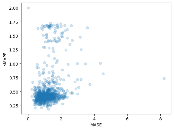

为了绘制任何时间序列的预测，我们定义了以下助手：

import matplotlib.dates as mdates

def plot(ts_index, mv_index):
    fig, ax = plt.subplots()

    index = pd.period_range(
        start=multi_variate_test_dataset[ts_index][FieldName.START],
        periods=len(multi_variate_test_dataset[ts_index][FieldName.TARGET]),
        freq=multi_variate_test_dataset[ts_index][FieldName.START].freq,
    ).to_timestamp()

    ax.xaxis.set_minor_locator(mdates.HourLocator())

    ax.plot(
        index[-2 * prediction_length :],
        multi_variate_test_dataset[ts_index]["target"][mv_index, -2 * prediction_length :],
        label="actual",
    )

    ax.plot(
        index[-prediction_length:],
        forecasts[ts_index, ..., mv_index].mean(axis=0),
        label="mean",
    )
    ax.fill_between(
        index[-prediction_length:],
        forecasts[ts_index, ..., mv_index].mean(0)
        - forecasts[ts_index, ..., mv_index].std(axis=0),
        forecasts[ts_index, ..., mv_index].mean(0)
        + forecasts[ts_index, ..., mv_index].std(axis=0),
        alpha=0.2,
        interpolate=True,
        label="+/- 1-std",
    )
    ax.legend()
    fig.autofmt_xdate()

举个例子：

plot(0, 344)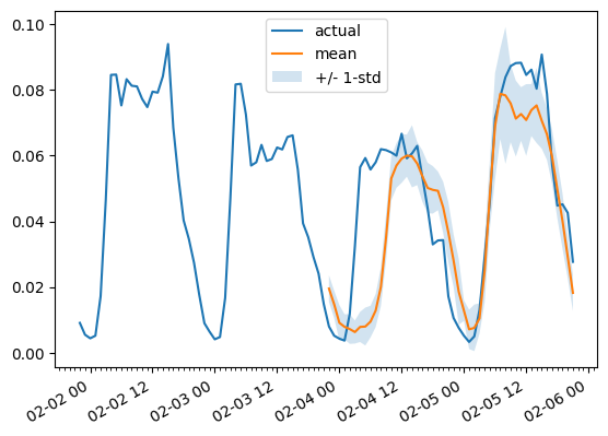

结论

我们如何与其他模型进行比较？ Monash Time Series Repository 有一个测试集 MASE 指标的比较表，我们可以将其添加到里面：

Dataset	SES	Theta	TBATS	ETS	(DHR-)ARIMA	PR	CatBoost	FFNN	DeepAR	N-BEATS	WaveNet	Transformer (uni.)	Informer (mv. our)
Traffic Hourly	1.922	1.922	2.482	2.294	2.535	1.281	1.571	0.892	0.825	1.100	1.066	0.821	1.191

可以看出，也许有些人会感到惊讶，多变量预测通常比单变量预测更差，原因是难以估计跨系列相关性/关系。估计增加的额外方差通常会损害最终的预测或模型学习虚假相关性。我们参考 这篇文章 来进一步阅读。当对大量数据进行训练时，多变量模型往往效果很好。

所以原始 Transformer 在这里仍然表现最好！将来，我们希望集中的更好地对这些模型进行基准测试，以便于重现几篇论文的结果。敬请期待更多！

资源

我们建议查看 Informer 文档 和 示例 notebook 链接在此博客文章的顶部。

赞赏

微信赞赏支付宝赞赏